Coloring India with logic programming
A language that doesn’t affect the way you think about programming, is not worth knowing - Alan Perlis
Every once in a while you come across a quote that pushes you to learn different languages that change the way you think about the problem not only from a theoretical perspective but also adds practical value to your toolbox so that you get to use the right tool for the right job. When I first started learning programming I created an Android app and I had to do some text parsing which was very cumbersome in Java and I get to learn Perl which I had used 5 minutes before to do some complex find and replace. Though I don’t get to use Perl daily and it adds practical value to my productivity. Some of the languages that we often hear among programmers that pushes the boundary are flavours of Lisp, statically typed functional programming languages like Haskell and so on. This post is about a different class of languages called logic programming languages that enabled me to express some complex problems with more concise and clear solutions.
Prolog introduction
Logic programming enables you to declare facts and lets you express the relation between the facts to arrive at the solution. Some examples of facts will be red is a color, leaves are green, John is a man, etc. But things are pretty useless if you cannot define the relation between the facts so that you can try to fit the given facts against the relation in order to see if there are any possible solutions. Let us take an example where we can define a man and a woman then we define a relationship between in order to see if they both like each other. The following are the facts :
- John is a man
- Kim is a woman
- John likes cats
- Kim likes cats
We can the define a good relationship when a man and a woman likes something in common in this case we have the facts and we try to constrain the given facts to see if we can match anything. The prolog code to declare the above facts is as below :
man(john).
man(george).
woman(kim).
likes(john, cats).
likes(kim, cats).
likes(george, dogs).
You can execute the programs at the online editor along with the tutorial instead of installing Prolog in your system :

We can ask questions to Prolog for the see if there is a fact in the database for the given value. Prolog will return true or false based on the value. The are entered in the query window of the above editor.
> man(john).
true
> man(adam).
false
On a similar note we can ask Prolog for the values that can fit in the fact or relation. We can ask the values of X that will is applicable to the given set of facts. When there is more than one match Prolog waits for the input to continue deducing more values for the variable. ; during printing solutions asks for more solutions and . exits the query.
> man(X).
X = john ;
X = george .
true
> woman(X).
X = kim .
true
> likes(john, X).
X = cats .
true
Prolog variables start with capital letters and hence cannot be used inside facts. As you can see Prolog facts are much more human readable and the facts doesn’t require any declaration like we do for a function in languages. We simply state the facts and we can state the relation as below :
relation(X, Y, Z) :- man(X), woman(Y), likes(X, Z), likes(Y, Z).
So a relation consists of three factors a man (X), a woman (Y) and something they like in common (Z). The rules indicated by comma signify that all the rules have to be satisfied in order to have the values for X, Y and Z. We declare the constraints and Prolog will try to replace some value of X such that it satisfies the fact. So X can have the values john and george. Similarly Y can only be kim. In a similar fashion let us define the common thing they like to be Z so X is a man who likes Z and Y is a woman who also likes Z. We try to fit george in this condition but there are no woman in the facts that likes dogs thus eliminating george to be a solution for X. In case of john he likes cats and we also have kim who also likes cats. Hence Prolog gives us the solution as X = john, Y = kim, Z = cats. The underlying method used to deduce the values is called unification. The query for the above follows the same as other examples
> relation(X, Y, Z).
X = john, Y = kim, Z = cats .
true
As you can see from the above Prolog makes us approach the problem from a very different perspective. Let me add one more powerful feature that we will be using to solve the coloring problem. One of the common problems is to figure out if we can reach from point A to B under some given constraints. So let us take the following facts that define the edges of a graph taking the points as the parameter
edge(a, b).
edge(b, c).
edge(c, d).
edge(d, e).
Now we need to define a relation to figure out whether we can go from A to E. Prolog allows us to define recursive rules
path(X, Y) :- edge(X, Y).
This is a simple rule where an edge between X and Y signifies the existence of a path between X and Y. But Prolog allows us to define Z such that it can be an intermediate point between X and Y. The below relation is such that X and Y can satisfy the fact that they can form an edge. Besides that we can have a point Z such that we have an edge from X to Z and Z itself can be a path to Y. Since we have the same rule defined twice it acts like an or operator.
path(X, Y) :- edge(X, Y).
path(X, Y) :- edge(X, Z), path(Z, Y).
The above definition is cool since we can try to verify a path from A to E and it starts with edge(a, e) which is invalid. It tries the other branch where edge(a, b) is true but we still don’t know whether path(Z, Y) can be true and hence Prolog tries with path(b, e) and moves on to have edge(b, c), path(c, e) and it reaches the point where we have path(d, e) which is true since there is an edge between D and E but the other branch cannot be satisfied since there are no further points beyond E and since it’s an or operator it returns true and then path(a, e) -> path(b, e) -> path(c, e) -> path(d, e) all return true thus satisfying the base assumption of the route A to E. This is a powerful example that tells us how we can model the same problem in a different way writing much easier and maintainable solutions.
In order to verify the false case we can try from B to A. We can imagine the call stack as path(b, c) -> path(c, d) -> path(d, e). There are no further paths or edges from E to A and hence it returns false thus making the base assumption of a path from B to A to be false.
core.logic introduction
This tutorial assumes that Clojure and lein are installed on your system. This post uses core.logic which is a port of MiniKaren library used for logic programming. Start a new project with lein new coloring-india and add the core.logic to your dependencies. You can still follow along as the Clojure examples are syntactically easier to understand.
(ns coloring-india.core
  (:require [clojure.core.logic :refer :all]
            [clojure.core.logic.fd :refer :all]
            [cheshire.core :refer :all]
            [clojure.core.logic.pldb :refer :all]))

(db-rel man name)
(db-rel woman name)
(db-rel likes name object)
The above code imports the functions for core.logic and JSON parsing along with declaring the relations. db-rel is a macro that takes the name of the fact as first argument followed by the arguments for the fact. We can declare a fact as below :
(db-fact (db) man 'john)
Since Clojure is immutable in nature this returns as a new DB with the update instead of mutating the DB. Clojure also provides us with the threading macro (->) that makes it easy to declare facts in these cases
(def facts
    (-> (db)
        (db-fact man 'john)
        (db-fact woman 'kim)
        (db-fact likes 'john 'cats)
        (db-fact likes 'kim 'cats)))
Now that we have the facts like the prolog example we can try to deduce some values for X and Y as below :
(run-db 1 facts [q]
        (fresh [X Y Z]
          (man X)
          (woman Y)
          (likes X Z)
          (likes Y Z)
          (== q [X Y Z])))

=> ([john kim cats])
Let us take it step by step run-db allows us to specify the number of results that need to be returned as first argument like limit on SQL statements. The second argument specifies the database against which the queries are run. Database in the sense some internal data structure that allows Prolog to store the facts to process them and not in SQL sense where we can interact with some other client. q is the query variable and we will get to this in a bit. Next we define three vars X, Y and Z which are called lvars (logical vars) similar to prolog. Then we define the constraints like the Prolog version. Then comes the part where we try to unify the values of X, Y and Z against. Think of it like an assignment statement in simpler terms. But unification forms the core part of core.logic and it’s beyond the scope of the tutorial. I highly recommend this excellent talk by David Nolen that explains the same. Now that we defined the constraints when we evaluate it this returns the result as ([john kim cats])
Similar to the prolog example Clojure also has conde which lets us define to recursive relationship between different goals. The prolog example above could be translated to below :
(pldb/db-rel edge start end)

(def facts
  (-> (pldb/db)
    (pldb/db-fact edge 'a 'b)
    (pldb/db-fact edge 'b 'c)
    (pldb/db-fact edge 'c 'd)
    (pldb/db-fact edge 'd 'e)))

(defn path
  [X Y]
  (conde
   [(edge X Y)]
   [(fresh [Z]
      (edge X Z)
      (path Z Y))]))

(run-db 1 facts [q]
        (fresh [X Y]
          (== X 'a)
          (== Y 'e)
          (path X Y)
          (== q [X Y])))

=> ([a e])

(run-db 1 facts [q]
        (fresh [X Y]
          (== X 'b)
          (== Y 'f)
          (path X Y)
          (== q [X Y])))

=> ()
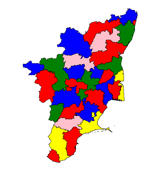
Coloring problem
As much as I was amazed by this declarative approach we also have an added advantage of the fact that it works in Clojure leveraging parallelism, rich data structure and code generation capabilities with macros. So I decided to solve the coloring problem with Clojure and logic programming. The coloring problem is a problem where we need to color the parts of a polygon in such a way that two adjacent parts don’t have the same color.
Finding adjacent districts
The first point was to get all the data we need to plot the parts on a map. I found a GeoJSON database for India and downloaded the whole set which comes around 30MB. Then with Python I derived all the coordinates of the form (latitude longitude district). This way we have all the latitude and longitudes for all the districts. We need to figure out whether two districts are adjacent to each other or not which can be deduced by the fact that they share a border and hence a set of same latitude and longitude values along the border. If they don’t share even a single point of same latitude and longitude then they cannot be adjacent districts. We also need to make sure that the district names themselves cannot be equal so that the district doesn’t match itself. Since all the conditions need to be matched and there is no recursive matching we have used all instead of conde. This can be expressed as a following goal :
(defn adjacent
  [district-a district-b]
  (all
   (fresh [latitude longitude]
     (coord latitude longitude district-a)
     (coord latitude longitude district-b)
     (!= district-a district-b))))
We can form the coordinates database using the JSON data as below. We get the file name and then load the JSON data forming a list of latitude, longitude and name. Thus this returns us the database for the given file after reduction. reduce can be thought of the fold function in other languages where we start with some accumulator here being DB and then we add the fact the returning updated DB which is used as the accumulator for further processing finally giving us the database.
(defn create-db
  [file]
  (let [res (->> file
                 io/resource
                 slurp
                 parse-string
                 (map (fn [[lat long name]] [lat long (keyword name)])))]
  (reduce
   (fn [db c]
     (apply pldb/db-fact db coord c))
   (pldb/db)
   res)))
Now with the given database we can construct a list of pairs that gives us all the adjacent districts as below. We run the query against the database and we also use run* which returns all the results. Here there is a catch that there might be both (A B) and (B A) which signify the same relation that A and B can be adjacent to each other. Thus we sort them to get ((A B) (A B)) and then perform distinct to get only ((A B)) :
(defn adjacent-districts
  [db]
  (->> (pldb/with-db db (run* [q]
                          (fresh [x y]
                            (adjacent x y)
                            (== q [x y]))))
       (map sort)
       distinct))
Now that we have adjacent districts in place we need to find the colors for them so that they don’t conflict each other. This can defined as below :
(defn neighbor
  [state-a state-b]
  (all
   (color state-a)
   (color state-b)
   (!= state-a state-b)))
We also generate the color database similar to the coordinates database. We shuffle the list and return n colors such that it is reduced to a database
(defn get-colors
  [n]
  (take n (shuffle ["red" "blue" "orchid" "sandybrown" "blue"])))

(defn generate-colors
  [n]
  (reduce (fn [db c]
            (pldb/db-fact db color c))
          (pldb/db)
   (get-colors n)))
Now that we have everything in place we need to define lvars for the district so that we can run it against the color database to get all the associations. But since we have varied number of steps we cannot handcode like X, Y and Z for 30 districts. So we generate a map of district name against an lvar and then use it
(defn generate-lvars
  [names]
  (zipmap (repeatedly lvar) names))

(def lvars (generate-lvars districts))

(def probs (mapv (fn [[x y]] (neighbor (x lvars) (y lvars))) adjacent))
Now that we have the color database and lvars along with the adjacent states we need to figure out the colors against the neighbor constraint so that we can get a JSON of district name and a color against the name to be plotted with D3.js . The final piece is as below :
(def sols (pldb/with-db colors (run 1 [q]
                                      (and* probs)
                                      (== q lvars)))
We combine all the constraints using and* which is similar to all and then unify against the query variable q which gives us the values of colors for all the districts such that two adjacent districts cannot have the same value.
Plotting with D3.js
D3.js provides support to plot geographical data in the form of maps. We can load the entire 30MB JSON with the co-ordinates and D3.js constructs SVG for each given district as a polygon and then during the SVG creation we can access the district name thus setting the appropriate color. To be honest I am still a beginner to D3.js and plotting in general. The library is so rich in nature that there are lot of cool things that we can do with it and it deserves a separate tutorial. The sample output is as below :
Great things
- Access to Clojure parallelism that enabled parallel processing on this project so that I can color different independent districts in parallel.
- Clojure also has rich data structures compared to Prolog that enables us to slice and dice the result to perform more post processing.
- REPL oriented programming enabled faster iteration where we can redefine the DB on the fly to see the results
Not so great things
Aside from all the cool things that can be done with logic programming it gives us a fresh breath of ideas and abstractions to play around with. But it is also not something magical in its working that there is no ecosystem around the logic programming community though a lot of cool things can be done with it. I also hit some scalability issues like I tried to unify the entire nation’s district around 600 lvars which caused the SWI-prolog implementation to segfault that reminds me of the fact that there is also a cost towards the abstractions that we leverage. Thus I was not able to completely solve the problem on country level and had to solve it for different states and combine the solutions together.
Conclusion
With enough being said logic programming has thought me to expand the horizons and also to express in more concise manner. It also kindles my curiosity to build something with other languages with different paradigms like stack based languages. Prolog is also not some toy tool for simpler demos and Prolog is used in production and I will link below to the videos that are worth a watch.
Thanks a lot to the Clojure community at Slack channel for their help and David Nolen for creating this library.